
Methods of yield programming and crop water consumption forecasting
23 min read
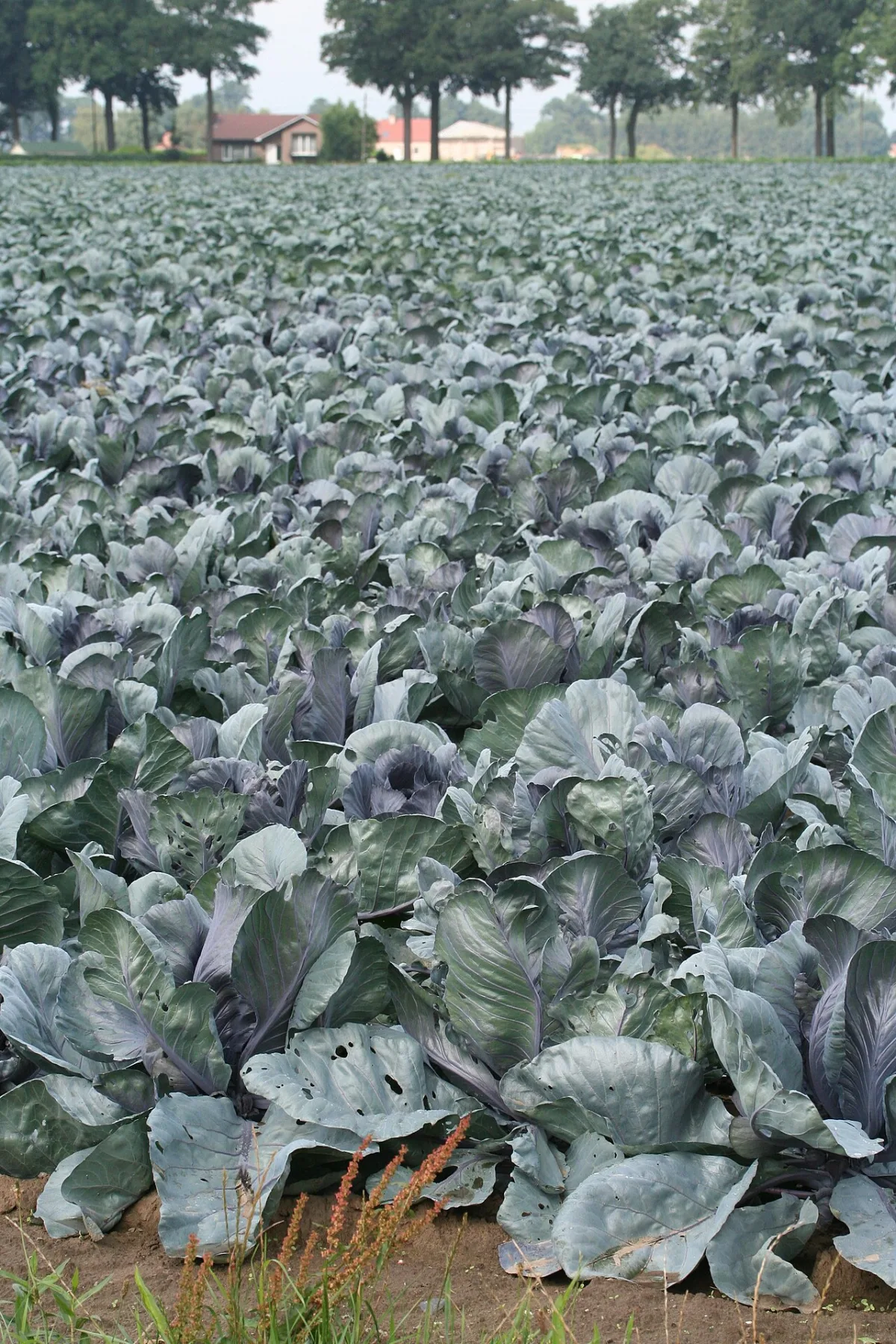
Crop yield programming involves calculating yield based on a pre-established program, taking into account physico-geographical, soil and agrometeorological conditions, and the biological characteristics of plants.
Crop yield programming is a complex process that includes a number of stages for building and using mathematical models to solve optimization and yield programming tasks: the maximum possible — based on incoming solar energy, the optimally possible — based on bioclimatic indicators of land productivity, and the potentially possible — based on crop moisture availability and the use of moisture by crops during the growing season.
The first attempts to use the properties of inertial natural processes, apply weather typing methods, the "analog year" concept, and the "weather-yield" dynamic model to optimize mineral nutrition of plants depending on the weather conditions of the growing season were made by A.R. Konstantinov, Kh.A. Tooming, and O.D. Sirotenko in the 1970s–1990s.
Over the last two decades, significant progress has been observed in the development of calculation models for establishing links in the "climate-soil-crop" system. Of interest is the simulation system "climate-yield" developed at the All-Russian Research Institute of Agricultural Meteorology (O.D. Sirotenko et al.) and some results of its application.
The main components of the system are: a complex of simulation models, an information database, a software package for building annual climate scenarios, and system support.
The foundation of the "climate-yield" simulation system is the applied dynamic model of energy-mass exchange and agroecosystem productivity developed by O.D. Sirotenko. The model is a closed system of differential equations integrated numerically with a daily time step throughout the growing season of the corresponding crop. The model is divided into three interconnected blocks, each solving a corresponding subsystem of equations to calculate: the dynamics of the agrobiocenosis phytomass of individual plant organs as a result of modeling the processes of photosynthesis, respiration, growth, development, and aging; the dynamics of soil moisture reserves as a result of modeling the processes of infiltration, evaporation, transpiration, and root water uptake; the dynamics of soil mineral nitrogen by modeling the processes of nitrification, denitrification, root uptake, and leaching.
The system's information database consists of annually updated monthly data on temperature and precipitation for the last 100 years, averaged by administrative regions and equivalent territorial units. Additionally, a five-year array of daily hydrometeorological data is used for tuning and verifying the models. The information database contains characteristics of the agrophysical and agrochemical properties of soils, as well as regional yield statistics for cereal crops for the post-war period.
Methodology for Stochastic Modeling of Meteorological Data
Future climate state scenarios generally contain information about changes in monthly temperature and precipitation values. Furthermore, the main hundred-year meteorological data array also contains only monthly temperature and precipitation values.
A stochastic model has been created that uses the Monte Carlo method to generate an ensemble of annual realizations of daily meteorological element complexes corresponding to specified monthly values. To reconstruct the initial averaged values of solar radiation and air humidity, statistical relationships between these variables and temperature and precipitation were used. A methodology was also developed to reconstruct initial values (as of the date of growing season resumption) for soil moisture reserves and available soil nitrogen content for each year.
The developed "climate-yield" system allowed for the first time the integration of hydrometeorological, agronomic, and soil property datasets covering the entire country with a powerful interpretive system in the form of a complex of models for energy-mass exchange and the productivity of the most important agricultural crops. The most significant identified regularity is the existence of two periods of growth in climatically determined yield — at the beginning of the 20th century (peaking in 1910–1920) and at present. The last minimum in the secular trend of yield occurred in years close to 1960, after which a steady and clearly expressed improvement in the growth conditions for cereal crops began.
Assessment of Bioclimatic Potential and Agrochemical Modeling
By assessing the country's current soil and climatic potential, it is possible to answer questions about its potential transformation under the influence of global warming. The results of calculations regarding expected productivity changes for two paleoclimatic analogs of global warming — the Holocene climatic optimum (HCO) and the Mikulino interglacial (MIG) — allow for the conclusion that climate evolution according to these two scenarios is generally favorable for agriculture. As an indicator of productivity, the focus is not on the yield of a specific agricultural crop, but on the total dry above-ground biomass productivity of a grassland agroecosystem over the period of the year with temperatures above 5°C, termed bioclimatic potential (BCP) according to D.I. Shashko.
We propose to consider an interesting solution to the problem of developing an optimal regime for increasing the productivity of arable land at the "Nizhegorodsky" Center for Agrochemical Service. A complex mathematical method for modeling the relationship between crop yield and agrochemical parameters of soil fertility and climatic conditions was chosen. The model system links the output parameter (response function) — the yield of winter and spring wheat, winter rye, and barley — with four main soil factors (content of humus, available phosphorus, exchangeable potassium, pH) and two climatic factors (G.T. Selyaninov's hydrothermal coefficient and the sum of positive temperatures (above 10°C)).
In the complex statistical-stochastic modeling, a multiplicative regression model of the dependence of the response function on regression factors was used. The regression coefficients of the nonlinear multiplicative forecast equation are determined by a complex algorithm, which includes:
- formation of the input data matrix;
- formation of the output parameter column;
- transposition;
- matrix inversion;
- multiplication of the transposed and then the inverted matrix by the output data column (yield), etc.
Methodology of mathematical yield modeling
Using the preliminary regression multiplicative equation, gross errors were estimated in the database where the relative forecast error exceeded 20%. Experimental yield values in such plots ("outliers") were replaced with theoretical forecast values. Based on the corrected yield database (output parameter column) and the unchanged matrix of the six input factors, the main nonlinear multiplicative regression forecast equation was formed.
The resulting equation can be used to assess the "heterogeneity" of the entire technology, determine the "influence functions" of each input factor on yield, and set "corridors" for input factors to achieve a programmed yield.
In accordance with the real parameters of the mean values and standard deviations of the input factors, a 6x300 two-dimensional array was formed, where 6 is the factor index and 300 is the index of the number of realizations of computer-technological "experiments" using the Monte Carlo method based on the main equation.
If all six factors changed simultaneously, the coefficient of variation of the response function characterized the "heterogeneity" of the entire technology. If five factors were fixed at a mean level, and elements of the array were introduced into the equation instead of the sixth factor, then the coefficient of variation of the response function characterized the influence of each input factor on yield.
According to the data from 14 reference plots, the calculated "heterogeneity" of the technology was 35%.
| Factor | Influence value |
| Exchangeable potassium content | 32.5% |
| Soil acidity | 36.5% |
The programming of cereal yields was carried out as follows: based on the specified yield value and its error obtained during computer realizations using the Monte Carlo method, the mean values and standard deviations of the input factors that ensure the programmed yield level are determined.
Practical application of statistical modeling
Thus, statistical-stochastic modeling allows for obtaining accurate (mathematically rigorous) nonlinear multiplicative regression equations and opens a path to solving many practical problems based on data from reference plots and field experiments:
- evaluate the reliability of initial information and the quality (fertility level) of soils;
- determine the degree of influence of each factor on crop yield, and the intervals of input factors for the programmed productivity of each field;
- forecast and program possible crop yield levels for given conditions on a computer;
- study the physiological features of the influence of soil factors on crop productivity;
- develop a methodology for the economic optimization of organic and mineral fertilizer application.
The introduction of an adaptive-landscape farming system into agricultural production involves the use of yield programming as an assessment indicator of the soil-climatic resources of a territory. This is the most important path for the rational practical application of the basic laws of farming and increasing the efficiency of solar energy utilization.
For an approximate assessment of the maximum or potential yield (PY), the formula of A.A. Nichiporovich can be used, which links potential yield with solar radiation:
109 R K biop - 102,4.103,102, where Ybiol is the biological yield of absolutely dry plant mass, centner/ha;
109 R - amount of incoming PAR during the growing season of the crop in a given zone, billion kcal/ha;
K - planned coefficient of PAR utilization, %;
102 - 100%; 4 10 s - amount of energy released during the combustion of 1 kg of dry biomass matter, kcal/kg;
102 - coefficient for converting kg to centners.
For example, spring wheat crops are programmed to assimilate 2% of PAR. During the growing season, about 2 billion kcal/ha falls on wheat crops. By substituting these values into the formula, we determine that under these conditions, 100 centner/ha of spring wheat dry matter can be obtained:
2 *10 9 *2% 1AA, u 100 centner/ha.
G\C\(77„ L 1 P 2
At the same time, to ensure high PAR efficiency for crops, it is necessary to comply with agrotechnical requirements for growing agricultural crops.
Solar heat, moisture, and soil conditions form a unified complex, the mathematical expression of which is integrated into the A.M. Ryabchikov formula, allowing for high-precision determination of the productivity of the optimally possible phytomass:
where KR is the biohydrothermal productivity potential, in points;
W is productive moisture (average annual precipitation P minus runoff S), in mm;
Tv is the growing season, in decades;
36 is the number of decades in a year;
R is the radiation balance over this period, in kcal/cm2.
This formula includes the arrival of integral radiation, which directly affects the evaporation of water from the surface of the soil and plants. For calculations, only productive moisture, which plants use for the formation of dry biomass, is usually introduced into the formula.
The bioclimatic productivity potential (BPP) of land is determined by the D.I. Shashko formula.
The bioclimatic potential (BPP) - the main indicator of yield - is calculated by the formula
BPP = Kr • P 1000 where Kr = l,151g(20Md) - 0,21 + 0,63Md - Md2;
Here Lt is the sum of air temperatures >10°C or >5°C depending on the limiting temperatures of a specific crop; P is the sum of precipitation for the period under consideration, in mm; d is the air humidity deficit, in mb; a is relative humidity of air">relative air humidity, %; 1a is saturated vapor pressure, in mb.
The dimensions of potential biological productivity can be converted into yield values for various crops according to the condition m = ^-BPP L 0,
K, where Kp is the crop productivity coefficient (yield per 100° sum of temperatures) according to empirical data.
According to the latter condition, the productivity of a specific crop can also be calculated if the BPP values are determined by the sums of temperatures for its growing season.
It should be noted that the influence of climate on plant productivity is refracted through the soil. Therefore, to the established points of its productive value, or relative BPP values, an adjustment for soil quality is required. Such a corrected score will characterize the soil quality (bonitet) against the background of specific climatic conditions.
The bioclimatic potential of a territory determines the zonal type of agricultural specialization, farming systems, and other features of agricultural production.
Theoretically possible plant yields depending on the moisture content in the soil and the amount of atmospheric precipitation during the growing season can be calculated using the I.V. Tsyganov formula. The model is convenient for calculations, and the number of parameters is sufficiently informative. Yield calculation (according to Tsyganov):
_(HB-WILT) + (0.5-P-10) г, m i ha ” where Y t/ha is the probabilistic theoretical yield; HB is the spring water reserve at the lowest water capacity in the meter layer of the soil, in t/ha;
WILT is the water reserve at the wilting point in the meter layer of the soil, in t/ha;
P is the average long-term precipitation, in mm;
0.5 is the coefficient of utility of summer precipitation;
10 is the conversion coefficient, mm to t/ha;
TC is the transpiration coefficient, in t/ha;
K is the ratio coefficient of main production to by-products.
For example, for Chernozem conditions with a spring water reserve in the meter layer of the soil equal to 3000 t/ha, wilting point in the same layer equal to 1200 t/ha, average long-term precipitation during the barley growing season equal to 250 mm, a barley transpiration coefficient equal to 534, and a grain-to-straw ratio of 1:2, the barley yield will be: y = (3000-1200) + (250-a5-10).1 t/ha,
It should be noted that a frequent reason for the gap between theoretically possible and practical yields lies in the low level of soil fertility, the quality of seed material, and the violation of agrotechnical requirements for the cultivation of agricultural crops.
One of the possible options for yield forecasting can be the V.G. Sychev model, which is implemented according to the following principles.
The productivity of agricultural plants depends on biological characteristics, soil fertility, agricultural techniques, and meteorological conditions. To make a decision on changing the structure of sown areas and redistributing farm resources, it is necessary to know what yield a particular crop will produce under the specific, changing weather conditions of a given year. Having such a forecast, one can solve issues regarding the structure of crops (choice of cultivar, seed sowing rate, fertilizer doses, etc.) and, taking into account the specifics of the year, actively influence the yield value. Solving these tasks depends on the timeliness of the incoming information, at least a month before the start of sowing. However, it is impractical to compile a yield forecast in accordance with a weather forecast. It is more reasonable, using meteorological data, to directly establish their connection with yield and other characteristics. The author has proposed a simulation model for forecasting the adjustment of crop areas (based on yield forecasts) for a given year according to the following scheme. A database is created containing statistical materials, experimental data from the Geographical network, and the Hydrometeorological Service. Variables: a large number of indicators of air temperature, precipitation amount, soil moisture reserves; nutrient content: nitrate nitrogen, available forms of potassium and phosphorus, nutrient uptake, utilization coefficients of nitrogen, phosphorus, and potassium from fertilizers and natural soil fertility; chemical composition of plants; level of agricultural techniques, crop rotation, cultivar.
The function is the harvest, for example, of winter wheat or potato. Matrices of correlation coefficients between the above-mentioned indicators and harvests were obtained, and factors most closely related to the harvest were selected. All of them were divided into two groups depending on the correlation coefficients: the first — r < 0.45; the second — r > 0.45.
For each group in each year, an integral indicator is determined:
where xi is a factor included in the given group;
Si is the standard deviation of the i-th factor; n is the number of factors in the group.
Integral indicators were grouped, creating analog years. To ensure that data from different years are comparable, factors were presented in proportions to the previous or subsequent year (relative values). The results obtained showed interesting patterns. For example, in the year preceding a "grain year," the nutrient utilization coefficients were higher than in other years, and the chemical composition of the plants also changed. It is generally accepted that the average utilization coefficients of mineral fertilizers' NPK mineral fertilizers by grain crops are 60% for nitrogen, 20% for phosphorus, and 70% for potassium, while in the subsequent year they are 10, 15, and 10%, respectively. However, fluctuations in nutrient utilization coefficients for nitrogen range from 30–85%, for phosphorus from 20–35%, and for potassium from 30–75%. Grain crops can absorb 20% of nitrogen, 5% of phosphorus, and 20% of potassium from the soil, although the extreme values of these coefficients also vary significantly depending on the crops, cultivar, agricultural practices, soil, and weather conditions, and, as the analysis results showed, they can serve as a forecast characteristic. The described scheme allows for the possibility of forecasting crop yield by years. The question of which variable factors are best to choose and what mathematical apparatus to apply remains to be decided. At this stage, the proposed scheme of computational forecasting using analog years should be considered an experiment and developed in this direction.
Methodology for establishing the dependence of yield on the water supply level of crops. An analysis of experimental data (including numerous foreign data) on the dependence of crop yield on the level of water supply indicates that the impact of a relative decrease in plant water supply on the relative decrease in their yield is not zonal, i.e., it has no territorial variability.
The most complete statistics in terms of quantity and quality exist regarding the links between yield and total crop water consumption.
The dependence of crop yield reduction on the level of their water supply for the case of uniform water deficit accumulation during the growing season is formalized in a generalized form by a parabolic curve.
In relative units of measurement, the analytical dependence has the following form: ∆Yi = A + B • ∆Evi + C • ∆Evi^2, where ∆Yi is the relative yield reduction as a fraction of the calculated (maximum, planned, project) yield;
∆Evi is the relative reduction in water supply (actual water consumption) of the crop as a fraction of the optimum.
The elements of equation (18) are determined as follows:
∆Evi = 1 - (Evi / Evopt), where Evopt is the optimal water consumption (evapotranspiration) at the optimal level of plant water supply, mm or m³/ha;
Evi is the water consumption at the actual water supply of plants, mm or m³/ha;
Yp is the yield at optimal plant water supply and implemented level of agricultural practices, c/ha or t/ha;
Ya is the actual crop yield under deficit water supply of plants, c/ha or t/ha.
It should be noted that optimal water consumption Evopt is observed when maintaining soil moisture reserves within the range from FC (field capacity) to a certain critical moisture content corresponding to the capillary rupture moisture (CRM).
For irrigated soils, the critical soil moisture βcr is approximately equal to:
βcr = 0.5 (βFC + βw), where βFC is the soil moisture content corresponding to field capacity, % by mass;
βw is the wilting moisture, % by mass.
In the present work, βcr (the threshold of permissible soil drying) is determined by the formula
βcr = 0.3614 + 1.476 W — 3.524 W^2, where W is the field capacity of the soil, mm.
When soil moisture drops below the critical level, plant water supply deteriorates, in accordance with which their yield decreases.
The optimal water consumption Evopt adopted in the calculations corresponds to the conditions of maintaining the moisture reserve in the root zone of the soil within the range from FC (field capacity) to a certain critical moisture content corresponding to the CRM (capillary rupture moisture).
The relative yield reduction (RYR) ∆Yi is determined by link equations. Differences between the established dependencies, which are cited in the works of domestic and foreign authors, are primarily explained by the quantity and quality of the experimental and statistical data used.
To establish the correlation equations between yield and irrigation rate, empirical parabolic equations have also been adopted. In this case, the total deficit of optimal water consumption is assumed to be equal to the optimal irrigation rate.
Using the correlation equations provided in Table 28, it is possible to determine the relative and absolute values of yield reduction resulting from a lack of water supply for other crops cultivated in the region. Calculation example 1. Relative yield reduction depending on the natural water availability of alfalfa for hay.
Zone Year Optimal water consumption, mm Natural water availability, mm Irrigation rate, mm Deficit of water consumption, mm Relative water deficit, A1 Relative yield reduction, AYi Yield, c/ha
Forest-steppe Moderately moist P=25% 490 140 350 0.25 0.15 13.5 76.5
Average P=50% 510 180 330 0.32 0.22 19.4 70.6
Moderately dry P=75% 560 250 310 0.45 0.36 32.6 57.4
Dry P=95% 610 350 260 0.55 0.51 45.8 44.2
If the optimal water consumption of a crop during the growing season is, AEV - water consumption deficit (irrigation rate), then natural water availability
In this case, the relative deficit of natural water availability is determined as A1 = 1 - Ev / Eopt.
Forest-steppe zone (Ku = 0.6).
Moderately dry year (75% probability).
Yield Ur = 90 c/ha.
According to the table 560 mm; AEV= 250 mm 560 - 250 = 310 mm.
E. D1P a £.= 1 -----Y- = 1 - ^ Y = 1 -0.5 5 5 = 0.4 4 5.
AYi = -0.002 +0.33-0.445+1.07(0.445)2=-0.002+0.147+0.212=0.36.
Thus, with a decrease in water availability for alfalfa by 44.5% from the optimal level, the hay yield will decrease by 36% from Ur and will amount to
Ug = Ur (1 -AY 1) = 90-0.64 = 57.4 c/ha.
Alfalfa yield (avg. 90 c/ha) with a shortage of natural soil moisture (c/ha)
Fig. 27. Graphs of yield dependence on natural soil moisture
Calculation example 2. Relative yield reduction of alfalfa with a decrease in irrigation rate compared to the optimal one in years with different humidity (Ural Federal District, forest-steppe zone)
Zone Year Water consumption, mm Irrigation rate, mm
Forest-steppe Moderately moist P=25% 360 90 Ku = 0.51-0.65 Average P=50% 530 160
Moderately dry P=75% 580 240
Dry P=95% 640 350
Average yield value 90 c/ha.
AEvi - reduction of irrigation rate;
Ayi - relative yield reduction;
relative reduction of water supply;
Ug = -0.002+0.33 07 2 - correlation equation.
The calculation sequence is presented in Table 29. Column 1 shows the gradation of the relative reduction of the optimal irrigation rate by 0.1, i.e., every 10%; column 2 shows the residual water supply for years with 25, 50, 75, and 95% probability respectively; column 3 shows the relative reduction of water supply A/vz. Based on the correlation equation for alfalfa, the relative yield reduction yi (column 4) is determined depending on the reduction of the irrigation rate (water supply). Taking the average alfalfa yield under optimal water supply of 90 c/ha, the actual yield reduction (column 5) was calculated, and column 6 shows the expected yield in c/ha.
Based on the calculation results, graphs were plotted, which are shown in Fig. 28.
Table 29
Relative reduction of irrigation rate Relative water supply reduction Relative yield reduction Actual yield reduction (c/ha) Yield (c/ha)
1 2 3 4 5 6
0.1 351 514 556 605 0.03 0.03 0.04 0.05 0.01 0.01 0.02 0.02 1.0 1.2 1.6 2.1 89.0 88.8 88.4 87.9
0.2 342 498 532 570 0.05 0.06 0.08 0.11 0.02 0.03 0.04 0.05 1.9 2.3 3.3 4.6 88.1 87.7 86.7 85.4
0.3 333 482 508 535 0.08 0.09 0.12 0.16 0.03 0.04 0.06 0.08 2.9 3.7 5.4 7.6 87.1 86.3 84.6 82.4
0.4 324 466 484 500 0.10 0.12 0.17 0.22 0.05 0.06 0.09 0.13 4.1 5.2 7.7 11.3 85.9 84.8 82.3 78.7
0.5 315 450 460 465 0.13 0.15 0.21 0.27 0.06 0.08 0.12 0.17 5.4 6.9 10.4 15.5 84.6 83.1 79.6 74.5
0.6 306 434 436 430 0.15 0.18 0.25 0.33 0.08 0.10 0.15 0.23 6.8 8.7 13.5 20.3 83.2 81.3 76.5 69.7
0.7 297 418 412 395 0.18 0.21 0.29 0.38 0.09 0.12 0.19 0.29 8.3 10.8 16.9 25.7 81.7 79.2 73.1 64.3
0.8 288 402 388 360 0.20 0.24 0.33 0.44 0.11 0.14 0.23 0.35 10.0 13.0 20.6 31.6 80.0 77.0 69.4 58.4
0.9 279 386 364 325 0.23 0.27 0.37 0.49 0.13 0.17 0.27 0.42 11.7 15.4 24.6 38.1 78.3 74.6 65.4 51.9
1.0 270 370 340 290 0.25 0.30 0.41 0.55 0.15 0.20 0.32 0.50 13.6 17.9 29.0 45.2 76.4 72.1 61.0 44.8
Yield losses (90 c/ha) with a decrease in irrigation rate
Fig. 28. Yield dependence on the reduction of the irrigation rate
The data in Table 30 is recommended as the basic methodological premise for solving the problem in a specific natural region. The given dependencies are averaged, therefore, under specific natural conditions, they can be adjusted taking into account local soil and climatic features.
Correlation equation Crop Probability P, %
Cereals (small grain) 50 AYi = 0.005 + 0.04 AXi + 0.079 AXi2
75 AYi = -0.006 + 0.153 AXi + 0.095 AXi2
95 AYi = 0.002 + 0.160 AXi + 0.205 AXi2 Late cabbage 50 AYi = -0.001 + 0.183 AXi + 0.106 AXi2
75 AYi = 0.010 + 0.260 AXi + 0.170 AXi2
95 AYi = -0.004 + 0.490 AXi + 0.205 AXi2
Forest-steppe zone Alfalfa for hay 50 AYi = -0.001 + 0.128 AXi + 0.117 AXi2
75 AYi = -0.003 + 0.225 AXi + 0.159 AXi2
95 AYi = 0.007 + 0.203 AXi + 0.356 AXi2
Cereals (small grain) 50 AYi = 0.004 + 0.234 AXi + 0.072 AXi2
75 AYi = -0.003 + 0.324 AXi + 0.186 AXi2
95 AYi = 0.006 + 0.326 AXi + 0.235 AXi2 Late cabbage 50 AYi = -0.004 + 0.311 AXi + 0.155 AXi2
75 AYi = -0.001 + 0.425 AXi + 0.265 AXi2
95 AYi = 0.002 + 0.561 AXi + 0.303 AXi2
Temperate steppe zone Alfalfa for hay 50 AYi = -0.006 + 0.159 AXi + 0.330 AXi2
75 AYi = -0.005 + 0.274 AXi + 0.352 AXi2
95 AYi = 0.014 + 0.267 AXi + 0.595 AXi2
Cereals (small grain) 50 AYi = 0.013 + 0.274 AXi + 0.277 AXi2
75 AYi = 0.011 + 0.365 AXi + 0.420 AXi2
95 AYi = 0.002 + 0.510 AXi + 0.477 AXi2
Late cabbage 50 AYi = -0.021 + 0.630 AXi + 0.193 AXi2
75 AYi = -0.016 + 0.779 AXi + 0.293 AXi2
95 AYi = -0.031 + 0.914 AXi + 0.277 AXi2
Dry steppe zone Alfalfa for hay 50 AYi = 0.021 + 0.177 AXi + 0.542 AXi2
75 AYi = -0,0 1 6 + 0,277 M i + 0,598 A X i 2
95 AYi = 0,011 + 0,335 M i + 0,761 A X i 2 Cereal crops 50 AYi = 0,005 + 0,409 M i + 0,367 A X i 2
75 AYi = 0,009 + 0,502 M i + 0,485 A X i 2
95 AYi = -0,009 + 0,693 M i + 0,542 A X i 2
Continuation of Table 30 Agricultural Provision
Correlation equation crop level P, % Late cabbage 50 AYi =-0,017+0,701 ■AXi + 0,269 A X i2
75 AYi =- 0,035 + 0,895 -AXi + 0,216AX i2
95 AYi =- 0,031 + 0,954-AXi + 0,333 A X i2
Note. Based on the work materials. Base equation: AYi = а сА Хг, where AYi is the relative yield reduction (in fractions of the calculated relative reduction of the irrigation rate (in fractions of the optimal); a, b, c are the equation parameters.
Read next
Irrigation For agronomists
The impact of global climate change on the development of agroecosystems in Russia

Irrigation For agronomists
Methods for planning and operational management of crop irrigation regimes
Irrigation For agronomists