
Methodology for conducting soil agrochemical surveys and compiling cartograms
8 min read
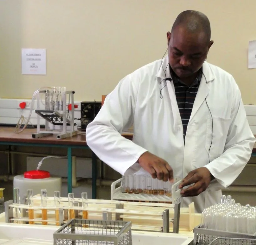
Agrochemical soil testing is the foundation for calculating the return on investment of mineral nutrition. Without accurate data on acidity and the content of mobile elements in each field, it is impossible to develop an effective fertilizer system. Periodic testing allows the agronomist to precisely dose nutrients, avoiding unnecessary costs and protecting the crop from nutrient deficiencies.
Preparation for testing and field partitioning
Before beginning field operations, collect the farm's historical data. You will need a land use plan with field boundaries, a soil map, a field history record book, as well as information on applied fertilizers and yields for the last 3 years. Prepare 4–5 working copies of the land use plan. Together with a representative of the agrochemical laboratory, inspect all lands and overlay a grid of elementary plots onto the maps.
The size of an elementary plot depends on the variability of the soil cover. The higher the soil heterogeneity, the more frequently samples must be taken to obtain reliable analysis results. Plot boundaries are marked on the plan as rectangles or squares and are numbered consecutively in the top right corner of each quadrilateral.
| Soil type and crop rotation direction | Elementary plot area, ha |
|---|---|
| Chernozem soils in field crop rotations | 10–15 |
| Grey forest and sod-podzolic soils | 5–8 |
| Vegetable and farm-adjacent crop rotations | Approximately 2 times more frequent (compared to field ones) |
| Vegetable crop rotations under irrigation | 2–4 |
- Fertilizers for sampling throughout the season — up to 45–60 kg/ha of active ingredient
- Waiting period after high fertilizer doses — 1.5–2 months
- Proportion of sub-arable samples under irrigation — no more than 15%
If manure has been applied to the fields, samples can be taken throughout the entire growing season. However, strictly ensure that particles of organic fertilizer do not enter the soil sample, otherwise the analysis results will be distorted.
Collection of mixed samples and creation of cartograms
Grid marking in the field begins with installing stakes along the field boundaries. The first stake on cross-lines is placed at a distance of half the width of the elementary plot, and all subsequent ones — at a distance of its full width. For longitudinal boundaries, stakes are set at a distance equal to the full length of the elementary plot.
- Identify a zone with the predominant soil variety within the elementary plot for sampling.
- Divide the length of the plot into 10 sections to determine the distance between sampling points.
- Walk along the axis of the plot and take individual samples from 10 sites — 2 samples from each.
- Thoroughly mix all 20 individual samples in a clean bucket and take a composite sample from them.
- Place the sample into a bag and insert a label indicating the farm, crop rotation, field, crop, sample number, depth, date, and the name of the sampler.
- Dry the soil on sheets of paper to an air-dry state in a well-ventilated room, avoiding direct sunlight.
Soil samples are always taken to the full depth of the arable layer. On irrigated lands, samples from the sub-arable horizon are taken additionally, but their number must not exceed 15% of the total number of samples taken from the arable layer.
In the laboratory, the delivered samples are ground, sieved, and analyzed for salt extract pH, mobile phosphorus content, and exchangeable potassium. The obtained results are entered into a ledger and then transferred in pencil to the center of each plot on the copy of the plan. Elementary plots are colored according to their nutrient availability classes.
When creating a cartogram, adjacent plots of the same class are combined into a common contour if there are at least two of them. Isolated plots of a different class are colored according to the color of their nearest neighbors. Based on the cartograms and field history, an agrochemical report is compiled with practical recommendations for fertilizer application.
In agrochemical research, an important descriptive statistical characteristic such as the mean value of any trait is often used. The mean is a highly informative measure of the "central tendency" of an observed variable, especially if its confidence interval is reported. The confidence interval for the mean represents the range of values around the estimate where the "true" (unknown) mean of the population, trait, or experimental variant lies with a given confidence level.
To determine the arithmetic mean of any trait (x), for example, the stem height of the Liman rice cultivar, we conduct the necessary number of measurements (from 10 to 200 plants, depending on the purpose and nature of the experiment). A variation series of plant height values (10, 20, 50 cases) is compiled: 95, 85, 87, 91, 79, 83, 86, 82, 78, 89 cm. Then all values of the variation series are summed: 95+85+87+91+79+ +83+86+82+78 +89 = 855. Dividing the sum by the number of terms, we obtain the arithmetic mean value – 855:10 = 85.5 cm. These results can be obtained on a PC using program 6.0, etc. After entering the ten plant height measurement values into the statistical processing program, we obtain the following statistical values: arithmetic mean of plant height (x); standard error of the mean (Sx), coefficient of variation of the trait (V), standard deviation (), and the experimental error (precision) (m). A table of the statistical characteristics of the Liman cultivar regarding plant height is then compiled.
Table 230 – Characteristics of rice plants by height Error Mean Arithmetic (precision) Mean square Standard error (arithmetic) Coefficient of varia- tion
Plant height, cm 85.5 1.67 6.2 5.3 1.96
The value of the standard error of the mean (Sx) is used to assess how well the calculated arithmetic mean reflects the general population, showing the range within which the mean value may vary for different samples from the general population. In practice, this is denoted as 85.5 ± 1.67 cm. This means that the plant height of the Liman cultivar varies from the mean of the entire general population by 85.5+1.67 = 87.17 to 85.5–1.67 = 83.83 cm. Our sample of 10 plants varies from 83.83 to 87.17 cm. It should be noted that if the arithmetic mean is determined to be 85.5 cm, the standard error of the mean should be 1.67 cm (not 1.6 – this is not correct!).
The coefficient of variation, variability, etc., indicates the variability of plant height relative to the mean value (6.2 %). In statistical literature, it is denoted as variation). It is a relative measure of variability, expressed as a percentage, and always has a positive value. Variability is considered insignificant or low if the coefficient of variation does not exceed 10 %; moderate if its value is above 10% but less than 20%; and significant or high if it exceeds 20%. The larger the sample (measurements) in an experiment, the lower the coefficient of variation. Sometimes in practical work, the coefficient of variation can be 50-80-90-100-110 %. Such an experiment should be rejected.
The standard deviation characterizes the error that is allowed on average when considering the mean in its general population (σ). It is also sometimes called the standard error of the mean of a trait and always has a positive value. The value of the standard deviation squared (σ2) indicates the variance. Variance and standard deviation serve as the primary measures of variation and dispersion of the values of the studied trait.
The experimental error value shows the precision with which the experiment was conducted. For a field experiment, it is generally accepted that if the error is no more than 5 %, the experiment was conducted correctly and properly.
To prepare a scientific report after statistical processing, a table of traits with corresponding statistical characteristics can be compiled.
Table 231 – Characteristics of rice plants by quantitative traits Trait
Plant height, cm 70.7±1.51 6.1 4.8 1.9 Length of the main panicle, cm 13.4±0.31 7.2 1.0 2.3 Number of grains from the main panicle, pcs. 99.3±5.40 17.2 17.1 5.4 Number of empty spikelets in the panicle, pcs. 31.8±3.75 37.3 11.9 11.8 Number of spikelets (total) in the panicle, pcs. 131.3±5.64 13.6 17.8 4.3 Grain weight from the main panicle, g 2.3±0.19 25.9 0.6 8.2 Grain weight per plant, g 4.3±0.79 37.9 2.5 18.3 1000-grain weight, g 23.1±0.88 12.3 2.8 3.9
Similar summary tables can be compiled for any crop, for any trait, for any field, vegetation, or laboratory experiment, when determining the amount of nutrients in various soils, for different predecessors, and experimental variants.
Read next

Agrochemistry For students
Organization and methodology of conducting agrochemical field experiments
Ecology For students
Methods and means of water quality control for natural and waste water
Plant protection For agronomists